AES Correlation Power Analysis

This post is not an introduction to the AES algorithm itself. I assume the reader already knows the AES round structure: initial AddRoundKey, repeated SubBytes, ShiftRows, MixColumns, and AddRoundKey, then the final round.

The goal here is narrower: given power traces and the corresponding plaintexts, recover the AES-128 key with Correlation Power Analysis (CPA).

References:

• AES specification: FIPS 197
• CPA reference: Correlation Power Analysis with a Leakage Model

1. Attack Model

I assume we know two things.

1. A set of power traces measured while the device encrypts plaintext blocks.
2. The plaintext block used for each trace.

For AES-128, the first operation is:

where $P$ is the plaintext block and $K$ is the 16-byte AES-128 master key. The first round then applies SubBytes:

CPA uses this kind of key-dependent intermediate value. For each byte position, we try every possible key byte from 0x00 to 0xff, predict the intermediate value, convert it into a leakage estimate, and check which guess correlates best with the measured traces.

2. Trace Parsing

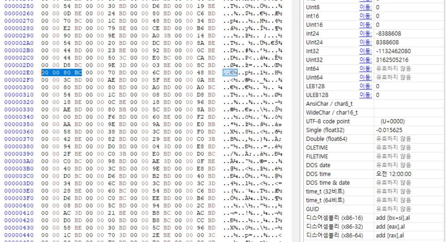
Before doing CPA, the trace data must be interpreted correctly. In this dataset the waveform is stored in 4-byte chunks. Looking at the bytes, values like 00 00 80 BC make sense as little-endian float32 samples. Interpreting them that way gives amplitudes in the same range as the plotted trace.

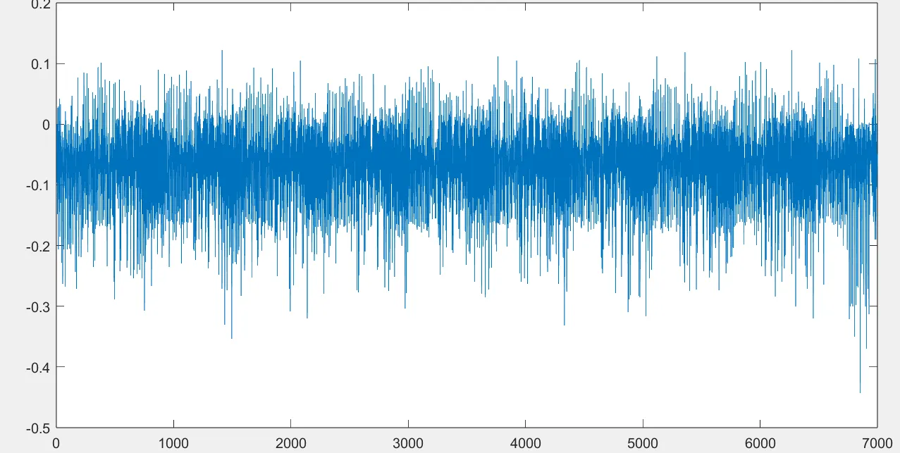
After parsing the samples, I first plot a single trace. A single trace is enough for Simple Power Analysis (SPA)-style sanity checks: AES should show repeated round-like activity, and the trace should not look like random decoded garbage.

CPA is a statistical attack across many traces, so alignment matters. If the same operation happens at different sample indices in different traces, the correlation peak is smeared out or disappears. Overlaying traces for different plaintexts is a quick way to check this.

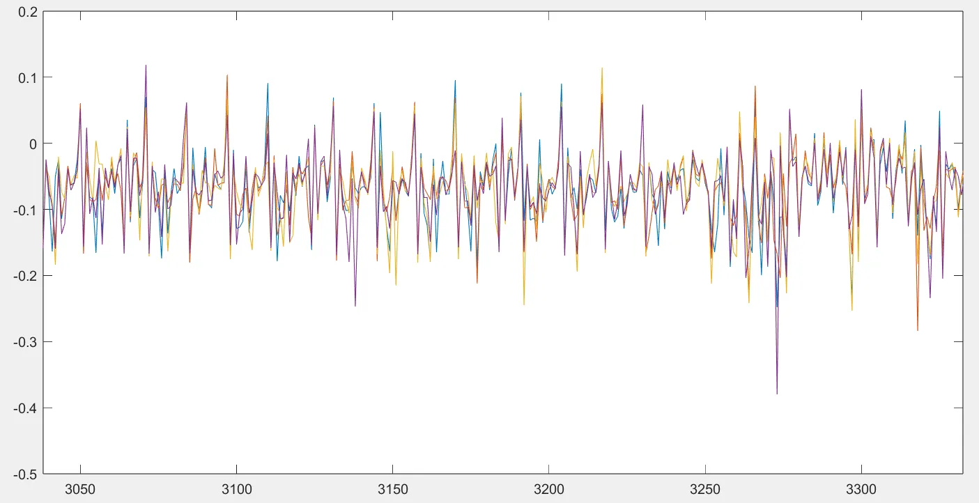
The traces above are reasonably aligned in the selected region. The next plot is the opposite case: the traces do not line up well, so a point-wise CPA would be much weaker unless the traces are realigned first.

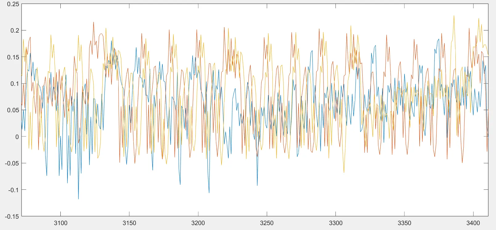
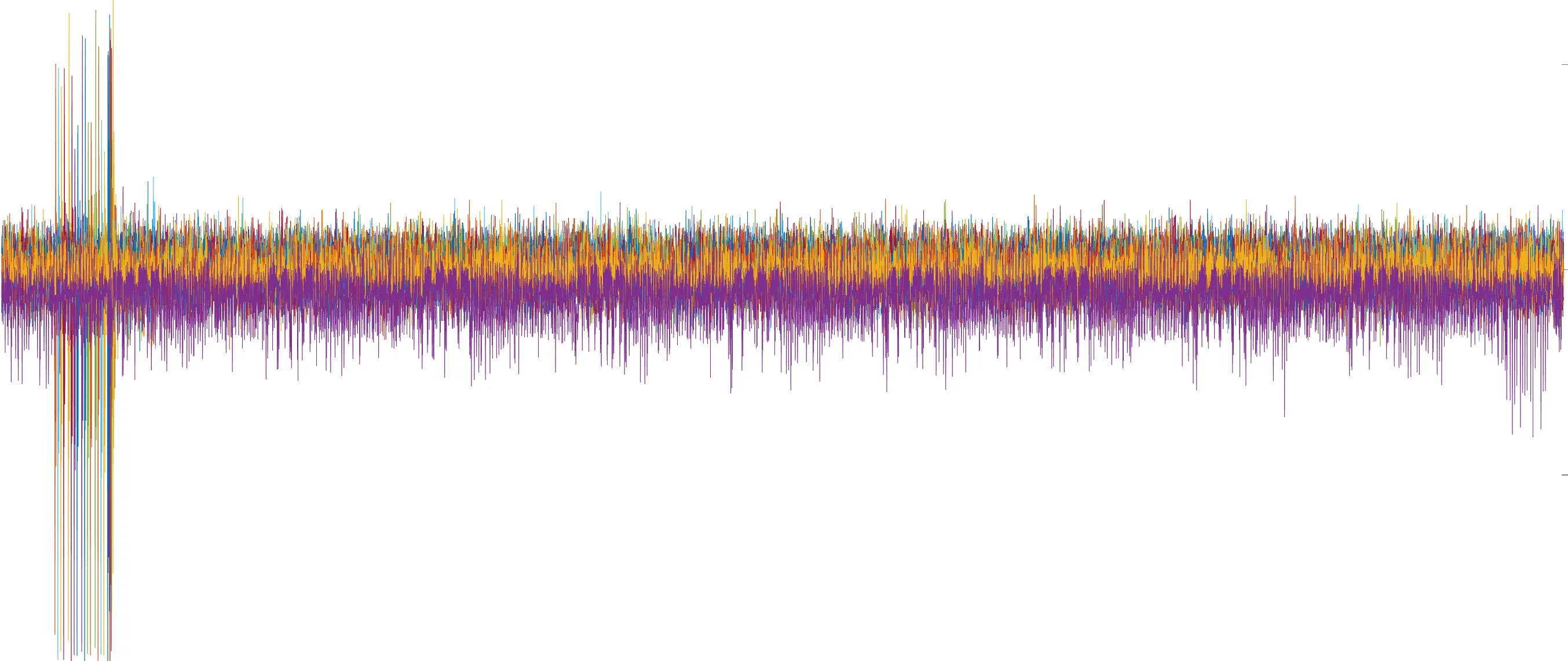
For a larger batch, a shared trigger or startup region is usually visible when many traces are drawn together. That region is useful for coarse alignment before zooming into the first AES round.

3. Choosing the Intermediate Value

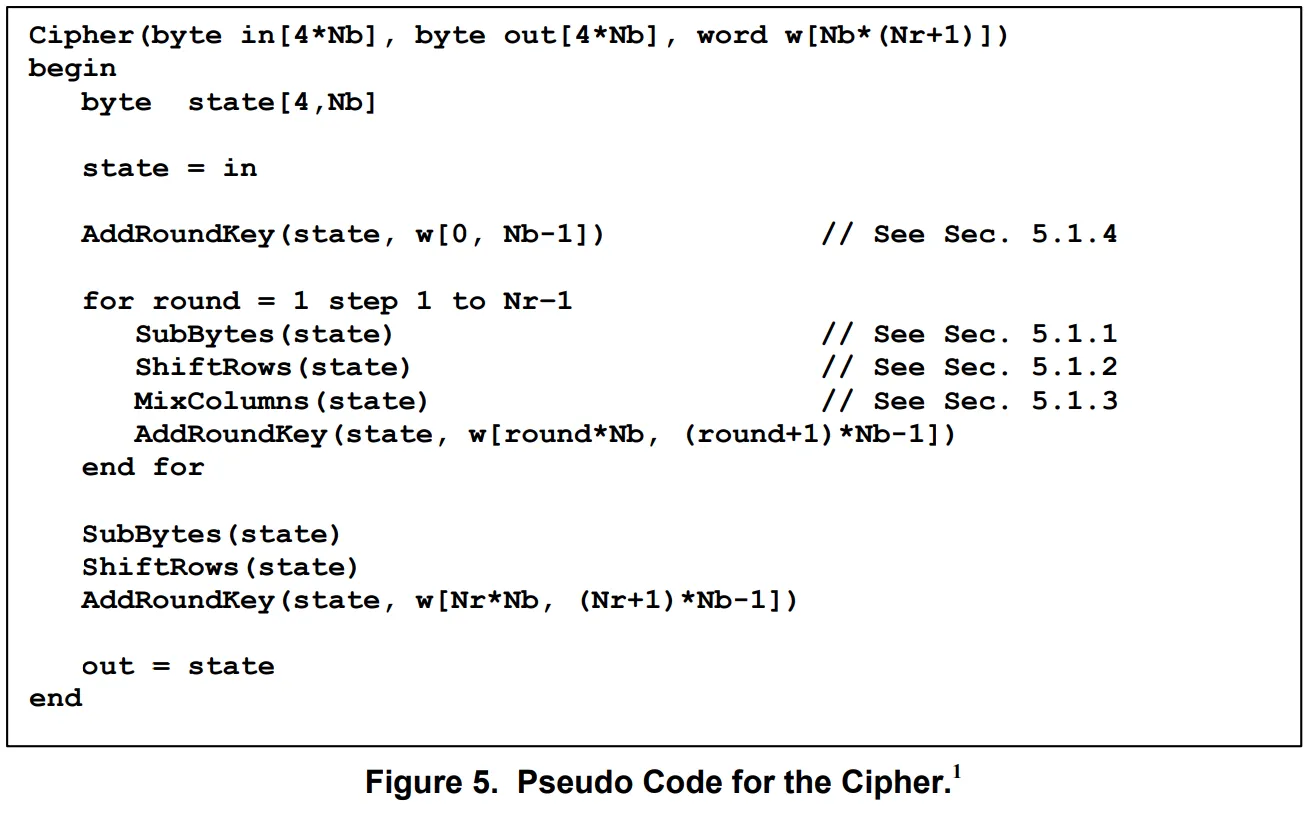
The AES encryption pseudocode begins with AddRoundKey, then enters the first round with SubBytes.

For byte position $b$, plaintext block $i$, and key-byte guess $k$, the first-round S-box target is:

Then I convert the target value into a leakage prediction. The simplest model is Hamming weight:

So for one byte position, each key guess produces one predicted leakage vector:

where $n$ is the number of traces.

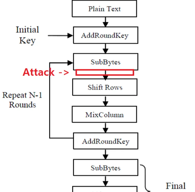
Targeting only AddRoundKey can work if the implementation leaks the absolute value of $P_i^{(b)} \oplus k$. In practice the first SubBytes output is usually a better target because it is nonlinear and key-dependent.

There is also an important leakage-model reason. If the measured leakage is closer to a transition from the plaintext byte to the AddRoundKey byte, the Hamming distance is:

For a fixed key guess, that value is constant across traces, so it cannot explain trace-to-trace variation. The S-box output gives a much more useful distribution.

For example, if the plaintext byte is 0xA0 and the key guess is 0x22:

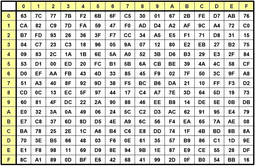
0xA0 ^ 0x22 = 0x82
Sbox[0x82] = 0x13

The Hamming weight of 0xA0 and 0x82 is both 2, so the raw XOR value may not create much visible separation in a simple model. After the S-box, the value changes nonlinearly. One sample does not prove the model, but across many plaintexts this nonlinear mapping gives the correct key guess a distinct correlation peak.

4. Correlation

Let $T_{i,t}$ be the measured power sample at time index $t$ in trace $i$. For each byte position $b$, key guess $k$, and time index $t$, compute the Pearson correlation between the predicted leakage vector and the measured samples at that time:

The attack loops over:

1. 16 byte positions.
2. 256 key guesses for each byte.
3. Every sample index in the trace window.

The recovered key byte is the key guess with the strongest absolute correlation peak:

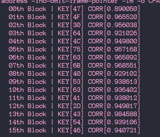
If the traces are clean and well aligned, the correct key guess often stands out very clearly.

The recovered 16 bytes match the AES key used by the implementation.

5. Reading the Correlation Trace

After computing CPA, it is useful to plot the correlation trace together with the original power trace. The peak should appear near the point where the targeted intermediate value is processed.

In this attack the target is the output of the first-round S-box. Therefore, a strong correlation peak around the first SubBytes activity is exactly what we expect.

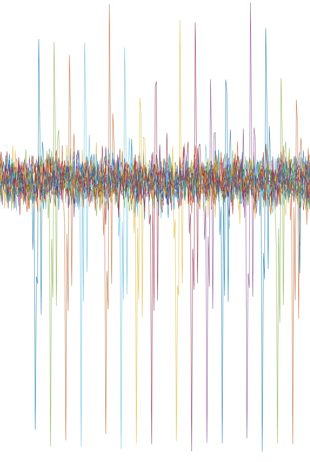
This plot is also a good debugging tool. If the best key guess is unstable or the peak appears in an impossible location, I would check the following first:

1. Endianness and sample type of the trace file.
2. Plaintext-to-trace pairing.
3. Trace alignment around the first round.
4. Whether the implementation uses a table, masked S-box, bitsliced S-box, or another leakage pattern.
5. Whether Hamming weight or Hamming distance is the better leakage model.

6. Core Implementation

The core of the attack is small. For each byte position and each key guess, compute:

for every trace $i$, then correlate that vector with each sample column of the trace matrix.

1
for (int byte_pos = 0; byte_pos < 16; byte_pos++) {
2
    for (int key = 0; key < 256; key++) {
3
        for (int trace_idx = 0; trace_idx < trace_count; trace_idx++) {
4
            uint8_t iv = Sbox[PT[trace_idx][byte_pos] ^ key];
5

6
            int hw = 0;
7
            for (int bit = 0; bit < 8; bit++) {
8
                hw += (iv >> bit) & 1;
9
            }
10

11
            predicted_hw[trace_idx] = hw;
12
        }
13

14
        correlate_against_trace_window(byte_pos, key, predicted_hw, traces);
15
    }
16
}

The important part is not the code shape, but the model:

Once this predicted leakage matches the real leakage at some sample index, the correct key-byte guess rises above the other 255 candidates.